Brian Cade published a scathing condemnation of current statistical practices in ecology. It promises to be highly influential; I have seen it cited by reviewers already. I agree with a great many points Brian raised. I also disagree with one very central point.
First let’s deal with the common ground. Brian’s assessment of how carelessly $AIC_c$ based model averaging is being used by ecologists is spot on. There’s a lot of sloppy reporting of results as well as egregiously misinformed conclusions. Perhaps the biggest issue with $AIC_c$ approaches is that they require thinking to be used effectively. In my experience with teaching ecologists to analyze data, they are desperate to avoid thinking, and it’s close cousin, judgement. They want a turn key analysis with a clear, unambiguous interpretation. Unfortunately that’s not what $AIC_c$ gives you.
Issues where Brian and I agree:
- Multi-collinearity among predictors is bad. Really bad. Worse than I thought.
- Model averaging including interaction terms is problematic.
- Using AIC weights to measure relative importance of predictors is a lousy idea.
- Using AIC model averaged coefficients to make predictions is just wrong.
- Model averaging predictions from a model set is always OK.
I’ll come back to each of those things below.
Is model averaging estimated coefficients legitimate?
Where I disagree with Brian is whether it makes sense to model average regression coefficients at all. Brian’s central point is that any degree of multi-collinearity between predictors causes the units of the regression coefficients to change depending on what other predictors are in the model. It is certainly true that the magnitude and even sign of a regression coefficient can change depending on which other predictors are in the model (this is the Frish-Waugh-Lovell Theorem). Brian’s assertion is that the units of the regression coefficients change between models as a result of this effect, and that means it is mathematically inappropriate to combine estimates from different models in an average. The consequences of the theorem are clearly correct; it is this latter interpretation of those effects that I disagree with.
As Brian did, I will start by examining the basic linear regression equation.
$$ E[y|x] = X \beta + \epsilon $$
$$ E[y|x] = X_1 \beta_1 + X_c \beta_c + \epsilon $$
The second equation partitions the predictors into a focal predictor $X_1$ and everything else, $X_c$. $\beta_1$ is a 1 x 1 matrix of the regression coefficient for $X_1$, and $\beta_c$ is a vector of regression coefficients for all the other predictors in $X_c$. When I look at that equation, it seems to me that the units of the products $X_1\beta_1$ and $X_c\beta_c$ have to be units of $y$. If that’s the case, then the units of $\beta_1$ are $y / X_1$. This might be the place where there is some deeper mathematics going on, so I am happy to be corrected, but as far as I can see the units of $\beta_1$ are independent of whatever $X_c$ is.
Next, Brian lays out several versions of the equation for $\beta_1$ to show how it is influenced by $X_c$. Maybe this is where the units change.
$$ \beta_{1,j} = \left(X’_1 M’_{C_j} M_{C_j} X_1\right)^{-1}X’_1 M’_{C_j} M_{C_j} y $$
$$ = Cov\left(M_{C_j}, X_1 y\right) / Var\left(M_{C_j} X_1\right) $$
$$ = \left(X’_1 X_1\right)^{-1} X’_1 y - \left(X’_1 X_1\right)^{-1} X’_1 X_{C_j} \beta_{C_j} $$
I find it easiest to think through the units of the third version. The first term has two parts. The units of $\left(X’_1 X_1\right)^{-1}$ are $X_1^{-2}$. The second part $X’_1 y$ has units of $X_1 y$. Put those together and you get $y X_1^{-1}$, the same units I found for $\beta_1$ above. The second term is pretty much identical except it has $X_{C_j}\beta_{C_j}$ instead of $y$, but the units of that matrix multiplication are $y$ anyway (see above). So that equation is dimensionally consistent and $\beta_1$ has units of $yX_1^{-1}$ as expected.
From that equation changing the components of $X_{C_j}$ will change the magnitude and possibly the sign of $\beta_1$. But not the units. So it is legitimate to average different values of $\beta_1$ across the models. It still might not be a good idea to do it when there is multi-collinearity, but not because the units change.
However, even if the magnitude and sign of the coefficient vary between models by a large amount, I think it is reasonable to examine a model averaged estimate of the coefficient as long as the variation is not due to including interaction terms in some of the models. The reason is that large variation between models will either lead to an increase in the model averaged standard error of the coefficient, or the offending model(s) will have a very small weight. In the first instance the model averaging procedure will in fact have told us exactly what we should conclude: conditional on this model set and data, we have poor information about the exact value of that coefficient. I will demonstrate using the simulated example that Brian created for habitat selection by sage grouse. It is important to point out that this example is designed to be problematic, and demonstrate the issues that arise with compositional covariates. Those issues are real. What I want to do here is check to see if model averaging coefficients in this highly problematic case leads to incorrect conclusions.
# all this data generation is from Cade 2015
library(tidyverse)
library(GGally)
# doesn't matter what this is -- if you use a different number your results will be different from mine.
set.seed(87)
df <- data_frame(
  pos.tot = runif(200,min=0.8,max=1.0),
  urban.tot = pmin(runif(200,min=0.0,max=0.02),1.0 - pos.tot),
  neg.tot = (1.0 - pmin(pos.tot + urban.tot,1)),
  x1= pmax(pos.tot - runif(200,min=0.05,max=0.30),0),
  x3= pmax(neg.tot - runif(200,min=0.0,max=0.10),0),
  x2= pmax(pos.tot - x1 - x3/2,0),
  x4= pmax(1 - x1 - x2 - x3 - urban.tot,0))

ggpairs(df)
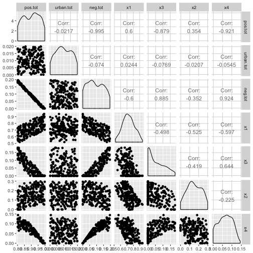
So there is a near perfect negative correlation between the things sage grouse like and the things they don’t like, although it gets less bad when considering the individual covariates. In fact, looking at the correlations between just x1 through x4 none of them have correlations bigger than $|0.7|$, so common “rules of thumb” would not exclude them. Now we’ll build up a Poisson response, and fit all the models
mean.y <- exp(-5.8 + 6.3*df$x1 + 15.2*df$x2)
df$y <- rpois(200,mean.y)

library(MuMIn)
globalMod <- glm(y ~ x1 + x2 + x3 + x4, data = df, na.action = na.fail, family=poisson())
fits <- dredge(globalMod)
## Fixed term is "(Intercept)"
options(digits = 2)
model.sel(fits)
## Global model call: glm(formula = y ~ x1 + x2 + x3 + x4, family = poisson(), data = df,
##     na.action = na.fail)
## ---
## Model selection table
##    (Intrc)    x1   x2    x3    x4 df logLik AICc  delta weight
## 4    -6.17  6.76 15.2              3   -379  764   0.00  0.271
## 15    0.54        8.4  -6.9  -6.7  4   -378  764   0.03  0.267
## 14    8.88 -8.42      -15.2 -15.3  4   -379  765   1.06  0.160
## 8    -5.64  6.23 14.7  -1.1        4   -379  766   1.84  0.108
## 16    2.50 -1.99  6.5  -8.9  -8.7  5   -378  766   2.03  0.098
## 12   -6.12  6.72 15.2        -0.1  4   -379  766   2.08  0.096
## 7     0.34        8.3 -10.9        3   -392  791  26.48  0.000
## 11    0.39        9.3       -11.3  3   -394  794  29.89  0.000
## 6     6.49 -5.94      -21.5        3   -441  887 122.82  0.000
## 3    -0.44       10.6              2   -458  919 154.87  0.000
## 10    8.30 -7.51            -26.4  3   -469  944 179.81  0.000
## 13    2.18            -12.4  -5.4  3   -523 1052 287.66  0.000
## 5     2.00            -15.5        2   -532 1069 304.49  0.000
## 9     2.28                  -15.2  2   -585 1175 410.63  0.000
## 2     2.15 -0.96                   2   -708 1421 656.42  0.000
## 1     1.46                         1   -712 1425 660.71  0.000
## Models ranked by AICc(x)
That’s some crazy stuff! Depending on which other variables are in the model, the coefficient for $x_1$ can even be negative. Using the common rule-of-thumb that I hate, there are 4 models with $\Delta AIC_c < 2$ and trying to explain why the coefficient of $x_1$ is sometimes positive and sometimes negative would cause some degree of heartburn.
Does looking at model averaged coefficients help? I only use the “full” average over all models.
ma_df <- model.avg(fits)
ma_coefs <- coefTable(ma_df, full=TRUE, adjust.se = TRUE)
coefnames <- row.names(ma_coefs)
ma_coefs <- as.data.frame(ma_coefs)
ma_coefs <- mutate(ma_coefs,
                   coefficient = coefnames,
                   t = Estimate / `Std. Error`,
                   p = pt(abs(t), df = 195, lower.tail = FALSE),
                   lower95 = Estimate - 1.96 * `Std. Error`,
                   upper95 = Estimate + 1.96 * `Std. Error`) %>% select(coefficient, Estimate, `Std. Error`, t, p, lower95, upper95)
knitr::kable(ma_coefs, digits = 2)
| coefficient | Estimate | Std. Error | t | p | lower95 | upper95 |
|---|---|---|---|---|---|---|
| (Intercept) | -1.1 | 5.8 | -0.18 | 0.43 | -12.4 | 10.3 |
| x1 | 1.6 | 5.8 | 0.28 | 0.39 | -9.8 | 13.1 |
| x2 | 10.1 | 5.9 | 1.72 | 0.04 | -1.4 | 21.5 |
| x3 | -5.3 | 5.9 | -0.89 | 0.19 | -16.8 | 6.3 |
| x4 | -5.1 | 6.0 | -0.85 | 0.20 | -16.9 | 6.7 |
In my opinion this tells us exactly what we want to know. The confidence intervals all include the true values, and all the coefficients have the correct sign. However, none of the confidence intervals exclude zero. This reflects the fact that conditional on this model set and data, there is not much information about habitat selection. This is a bit depressing given the strength of the effects and the sample size, but arises because of the strong multi-collinearity between predictor variables.
My estimate of the potential for multi-collinearity to make life difficult went way, way up after working through Brian’s examples. In particular, the naive application of pairwise correlation coefficients completely fails to detect the problem in this case. Where available, Variance Inflation Factors are better:
# unfortunately dredge() orders the models by AIC
# by default, so global model is 5
car::vif(get.models(fits, 5)[[1]])
##  x1  x2  x3  x4
## 201 147  39  38
So even though the pairwise correlation coefficients are not raising alarms, car::vif() does. This should always be run on the global model in the set before doing the $AIC_c$ analysis. Unfortunately car::vif() doesn’t work (directly) on many models of interest to ecologists.
Model Averaging including interaction terms
One place where model averaging coefficients really will get you in trouble is when there are interaction terms. The problem is that when there is an interaction term between $X_1$ and $X_i$, then the interpretation of $\beta_1$ shifts to be $y X^{-1}_{1}$ conditional on $X_2 = 0$. This can also lead to the magnitude of $\beta_1$ jumping around, and it is so frowned upon that many automatic model averaging functions will simply return an error if they detect the presence of an interaction.
Thinking about how the interpretation shifts in the presence of a different predictor is still not assuming the units change. The big difference between the discussion above and the effect of including an interaction is that in the presence of an interaction the interpretation of the coefficient is assuming a particular value of another covariate. Not just the presence of that covariate, but a specific value.
I think there is an easy fix to this problem. If all continuous covariates are centered, and all categorical predictors use sum-to-zero contrasts, then I think the interpretation of the individual coefficients does not change when interactions are present. But that’s mostly a guess. For now I recommend not model averaging coefficients when there are interactions present in some of the models. Model average the predictions from all the models if you really want help interpreting the model set.
Variable importance weights suck
Checkout the variable importance weights from the example above
importance(fits)
##                      x2   x1   x3   x4
## Importance:          0.84 0.73 0.63 0.62
## N containing models:    8    8    8    8
That doesn’t really help us at all. There isn’t much variation between them. The rank order matches the relative magnitude of the true coefficents. Just don’t do it.
Model averaging predictions
Brian points out, and I agree, that the solution to many model selection uncertainty conundrums is to model average the predictions. This avoids all the disagreements above completely, because the units of the response are always the units of the response, and everyone agrees on that! I much prefer model averaged predictions over almost anything else, if you’re using AIC~c~ based model selection.
One very large problem: do not ever (really, never), use model averaged coefficients to make model averaged predictions. This has nothing to do with the validity of model averaged coefficients. Rather, it is a consequence of the fallacy of non-linear averaging, AKA Jensen’s Inequality. The only time the model averaged coefficients will give the right answer for model averaged predictions is when the model is linear in the coefficients and the link between the linear predictor and the expected response is the identity function. In any other instance the answer will be wrong. Even if you are in that particular instance, getting the variance of the model averaged prediction from the coefficients is challenging. Both problems disappear if you just generate predictions from each model and then model average those.
Conclusion
IMO, it is legitimate to model average coefficients in some circumstances. There are many issues with interpretation and analysis when using $AIC_c$ in ecology, but let’s not throw the baby out with the bathwater.
