A sum-to-zero contrast codes a categorical variable as deviations from a grand mean. Social scientists use them extensively. Should ecologists?
EDIT the first version of this post that went up had some bugs in it. Hopefully all fixed now.
EDIT2 Annnd the second version still had bugs. Maybe fixed now.
More accurately, should I tell my students in Ecological Statistics to use them? Sum-to-zero contrasts are conceptually similar to centering a continuous variable by subtracting the mean from your predictor variable prior to analysis. Discussions of centering often end up conflated with scaling, which is dividing your predictor variable by a constant, usually the standard deviation, prior to analysis. Always scaling covariates prior to regression analysis is controversial advice. See for example Andrew Gelman’s blogpost and comments, or many crossvalidated questions such as this one which has links to many others. There is a good reference as well as some useful discussion in the comments of this question. In this post I focus on the effects of sum to zero contrasts for categorical variables and interactions with continuous variables.1
Here is my summary of the pros and cons of centering drawn from those references above.2
- Centering continuous variables eliminates collinearity between interaction and polynomial terms and the individual covariates that make them up.
- Centering does not affect inference about the covariates.
- Centering can improve the interpretability of the coefficients in a regression model, particularly because the intercept represents the value of the response at the mean of the predictor variables.
- Predicting out of sample data with a model fitted to centered data must be done carefully because the center of the out of sample data will be different from the fitted data.
- There may be some constant value other than the sample mean that makes more sense based on domain knowledge.
To make the discussion concrete, let me demonstrate with an example of the interaction between a continuous covariate and a categorical one. In the following I refer to the effect of individual covariates outside the interaction as the “simple effect” of that covariate.
data(iris)
m0 <- lm(Sepal.Width ~ Sepal.Length * Species, data = iris)
(summary_m0 <- summary(m0))
##
## Call:
## lm(formula = Sepal.Width ~ Sepal.Length * Species, data = iris)
##
## Residuals:
## Min 1Q Median 3Q Max
## -0.72394 -0.16327 -0.00289 0.16457 0.60954
##
## Coefficients:
## Estimate Std. Error t value Pr(>|t|)
## (Intercept) -0.5694 0.5539 -1.028 0.305622
## Sepal.Length 0.7985 0.1104 7.235 2.55e-11 ***
## Speciesversicolor 1.4416 0.7130 2.022 0.045056 *
## Speciesvirginica 2.0157 0.6861 2.938 0.003848 **
## Sepal.Length:Speciesversicolor -0.4788 0.1337 -3.582 0.000465 ***
## Sepal.Length:Speciesvirginica -0.5666 0.1262 -4.490 1.45e-05 ***
## ---
## Signif. codes: 0 '***' 0.001 '**' 0.01 '*' 0.05 '.' 0.1 ' ' 1
##
## Residual standard error: 0.2723 on 144 degrees of freedom
## Multiple R-squared: 0.6227, Adjusted R-squared: 0.6096
## F-statistic: 47.53 on 5 and 144 DF, p-value: < 2.2e-16The intercept of this model isn’t directly interpretable because it gives the average width at a length of zero, which is impossible. In addition, both the intercept and simple effect of length represent the change in width for only one species, setosa. The default contrast in R estimates coefficients for \(k - 1\) levels of a factor. In the simple effect of a factor each coefficient is the difference between the first level (estimated by the intercept), and the named level. In the above, Speciesversicolor has sepals that are 1.4 mm wider than setosa. The interaction coefficients
such as Sepal.Length:Speciesversicolor tell us how much the effect of Sepal.Length in versicolor changes from that in setosa. So every mm of sepal length in versicolor increases sepal width by \(0.8 - 0.48 = 0.32\) mm.
Maybe a plot will help.
library(ggplot2)
base_iris <- ggplot(iris, aes(x = Sepal.Length, y = Sepal.Width)) + geom_point(aes(shape = Species)) +
    xlab("Sepal Length [mm]") + ylab("Sepal Width [mm]")
library(broom)
nd <- expand.grid(Sepal.Length = seq(-1, 8, 0.1), Species = factor(levels(iris$Species)))
pred.0 <- augment(m0, newdata = nd)
base_iris + geom_line(aes(y = .fitted, linetype = Species), data = pred.0)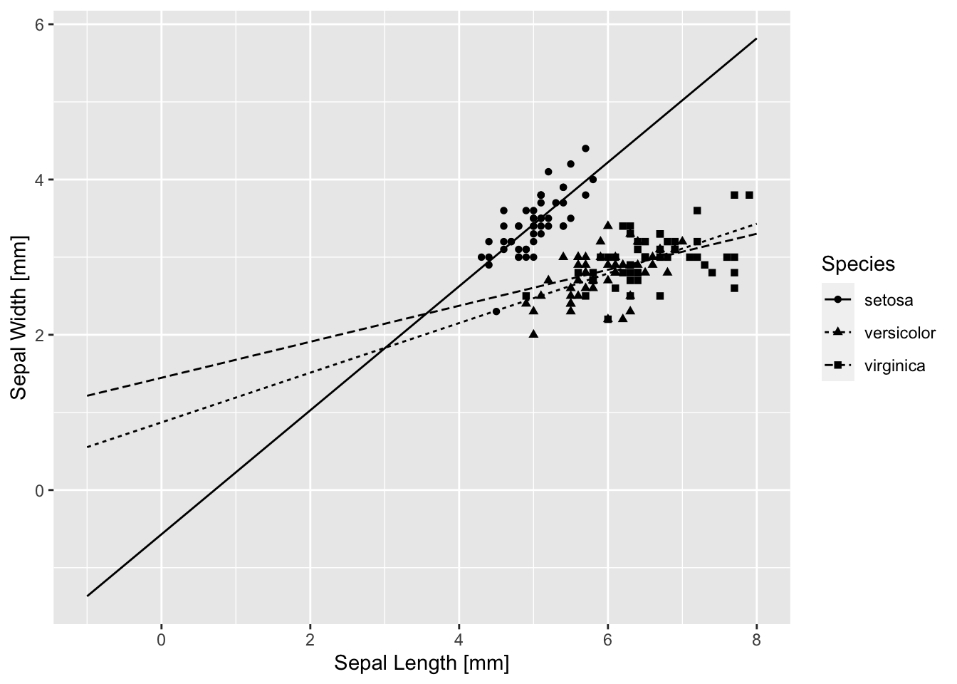
I did something rather silly looking there because I wanted to see where the curves cross x = 0. That is where the estimates for the intercept and simple effect of species are calculated. The intercept is negative, and the line for setosa crosses x = 0 well below y = 0. The simple effect estimates of Species are both positive, with virginica being larger, and indeed the line for virginica crosses x = 0 at the highest point. Similarly, the simple effect of length is the slope of the line for setosa, and it is larger than the slopes of the other two species because the estimated interactions are both negative. But not centering really makes things ugly for direct interpretation of the estimated coefficients.
Centering the continuous variable gives us
library(dplyr) #Stay in the tidyverse! ##
## Attaching package: 'dplyr'## The following objects are masked from 'package:stats':
##
## filter, lag## The following objects are masked from 'package:base':
##
## intersect, setdiff, setequal, unioniris <- iris %>% mutate(cSepal.Length = Sepal.Length - mean(Sepal.Length))
m1 <- lm(Sepal.Width ~ cSepal.Length * Species, data = iris)
(summary_m1 <- summary(m1))##
## Call:
## lm(formula = Sepal.Width ~ cSepal.Length * Species, data = iris)
##
## Residuals:
## Min 1Q Median 3Q Max
## -0.72394 -0.16327 -0.00289 0.16457 0.60954
##
## Coefficients:
## Estimate Std. Error t value Pr(>|t|)
## (Intercept) 4.0966 0.1001 40.916 < 2e-16 ***
## cSepal.Length 0.7985 0.1104 7.235 2.55e-11 ***
## Speciesversicolor -1.3563 0.1075 -12.616 < 2e-16 ***
## Speciesvirginica -1.2953 0.1165 -11.114 < 2e-16 ***
## cSepal.Length:Speciesversicolor -0.4788 0.1337 -3.582 0.000465 ***
## cSepal.Length:Speciesvirginica -0.5666 0.1262 -4.490 1.45e-05 ***
## ---
## Signif. codes: 0 '***' 0.001 '**' 0.01 '*' 0.05 '.' 0.1 ' ' 1
##
## Residual standard error: 0.2723 on 144 degrees of freedom
## Multiple R-squared: 0.6227, Adjusted R-squared: 0.6096
## F-statistic: 47.53 on 5 and 144 DF, p-value: < 2.2e-16Estimates and t-statistics for the continuous covariate, including the interaction terms, do not change. The t-statistics for the intercept and simple effect of species do change because now the model estimates the differences between the species at the mean length.
zapsmall(summary_m1$coefficients[, 3] - summary_m0$coefficients[, 3])## (Intercept) cSepal.Length
## 41.94445 0.00000
## Speciesversicolor Speciesvirginica
## -14.63795 -14.05196
## cSepal.Length:Speciesversicolor cSepal.Length:Speciesvirginica
## 0.00000 0.00000That’s OK, because they are really testing something quite different from before. Just to confirm that the graph isn’t different.
# remember to center the newdata values by the original mean!
nd <- nd %>% filter(Sepal.Length > 4) %>% mutate(cSepal.Length = Sepal.Length -
    mean(iris$Sepal.Length))
pred.1 <- augment(m1, newdata = nd)
base_iris + geom_line(aes(y = .fitted, linetype = Species), data = pred.1)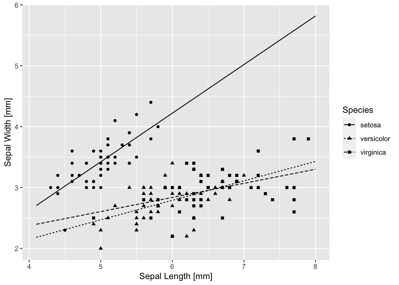
What happens if we use sum to zero contrasts for species?
iris$szSpecies <- iris$Species
contrasts(iris$szSpecies) <- contr.sum(3)
m2 <- lm(Sepal.Width ~ cSepal.Length * szSpecies, data = iris)
(summary_m2 <- summary(m2))
##
## Call:
## lm(formula = Sepal.Width ~ cSepal.Length * szSpecies, data = iris)
##
## Residuals:
## Min 1Q Median 3Q Max
## -0.72394 -0.16327 -0.00289 0.16457 0.60954
##
## Coefficients:
## Estimate Std. Error t value Pr(>|t|)
## (Intercept) 3.21278 0.04098 78.395 < 2e-16 ***
## cSepal.Length 0.45005 0.04900 9.185 4.11e-16 ***
## szSpecies1 0.88386 0.07086 12.473 < 2e-16 ***
## szSpecies2 -0.47240 0.04680 -10.094 < 2e-16 ***
## cSepal.Length:szSpecies1 0.34848 0.08038 4.335 2.72e-05 ***
## cSepal.Length:szSpecies2 -0.13033 0.06553 -1.989 0.0486 *
## ---
## Signif. codes: 0 '***' 0.001 '**' 0.01 '*' 0.05 '.' 0.1 ' ' 1
##
## Residual standard error: 0.2723 on 144 degrees of freedom
## Multiple R-squared: 0.6227, Adjusted R-squared: 0.6096
## F-statistic: 47.53 on 5 and 144 DF, p-value: < 2.2e-16I can now directly interpret the intercept as the average width at the average length, averaged over species. Similarly the simple effect of length as the change in width averaged across species. This seems like a very useful set of coefficients to look at, particularly if my categorical covariate has many levels. You might ask (I did), what do the categorical coefficients mean? They represent deviations from the mean intercept for each species. But what is species 1 and species 2? With sum to zero contrasts those coefficient refer to the first k-1 levels, so species 1 is setosa and species 2 is versicolor. OK, you say (I did), then where’s species virginica? After much head scratching, the answer is that it is the negative of the sum of the other two coefficients.
I just thought of something else. Are those “average” intercept and slope the same as what I would get if I only use cSepal.Length?
m3 <- lm(Sepal.Width ~ cSepal.Length, data = iris)
(summary_m3 <- summary(m3))
##
## Call:
## lm(formula = Sepal.Width ~ cSepal.Length, data = iris)
##
## Residuals:
## Min 1Q Median 3Q Max
## -1.1095 -0.2454 -0.0167 0.2763 1.3338
##
## Coefficients:
## Estimate Std. Error t value Pr(>|t|)
## (Intercept) 3.05733 0.03546 86.22 <2e-16 ***
## cSepal.Length -0.06188 0.04297 -1.44 0.152
## ---
## Signif. codes: 0 '***' 0.001 '**' 0.01 '*' 0.05 '.' 0.1 ' ' 1
##
## Residual standard error: 0.4343 on 148 degrees of freedom
## Multiple R-squared: 0.01382, Adjusted R-squared: 0.007159
## F-statistic: 2.074 on 1 and 148 DF, p-value: 0.1519Whoa! It is not the same, in fact it is radically different. Totally different conclusion about the “average” effect.
m4 <- lm(Sepal.Width ~ cSepal.Length + szSpecies, data = iris)
(summary_m4 <- summary(m4))
##
## Call:
## lm(formula = Sepal.Width ~ cSepal.Length + szSpecies, data = iris)
##
## Residuals:
## Min 1Q Median 3Q Max
## -0.95096 -0.16522 0.00171 0.18416 0.72918
##
## Coefficients:
## Estimate Std. Error t value Pr(>|t|)
## (Intercept) 3.05733 0.02360 129.571 < 2e-16 ***
## cSepal.Length 0.34988 0.04630 7.557 4.19e-12 ***
## szSpecies1 0.66363 0.05115 12.974 < 2e-16 ***
## szSpecies2 -0.31976 0.03364 -9.504 < 2e-16 ***
## ---
## Signif. codes: 0 '***' 0.001 '**' 0.01 '*' 0.05 '.' 0.1 ' ' 1
##
## Residual standard error: 0.289 on 146 degrees of freedom
## Multiple R-squared: 0.5693, Adjusted R-squared: 0.5604
## F-statistic: 64.32 on 3 and 146 DF, p-value: < 2.2e-16This is closer to the conclusion obtained with the interaction model.
I have seen assertions in some papers (particularly from social sciences), that using sum to zero contrasts (also called effects coding, I believe), allows the direct interpretation of lower order terms in an ANOVA table even in the presence of interactions.
anova(m2) # doesn't matter which model I use## Analysis of Variance Table
##
## Response: Sepal.Width
## Df Sum Sq Mean Sq F value Pr(>F)
## cSepal.Length 1 0.3913 0.3913 5.2757 0.02307 *
## szSpecies 2 15.7225 7.8613 105.9948 < 2.2e-16 ***
## cSepal.Length:szSpecies 2 1.5132 0.7566 10.2011 7.19e-05 ***
## Residuals 144 10.6800 0.0742
## ---
## Signif. codes: 0 '***' 0.001 '**' 0.01 '*' 0.05 '.' 0.1 ' ' 1If so, in this case I could say “Sepal Width differs significantly between species.” I’m not sure I believe that. The ANOVA table is identical between all 3 models, whether I use sum-to-zero contrasts or not. Why should the interpretation differ if I just change the parameterization of the model?
Explaining treatment contrasts to students is a pain. I’m not sure that these are any easier. I have a few thoughts about the effects of sum-to-zero contrasts and model averaging, but that will have to wait for a different post.
All the code for this post, including that not shown, can be found here.↩︎
This stuff first appeared as a question on CrossValidated, but received no attention.↩︎
