Checking linear model assumptions

Many years ago I started making videos of my lectures for my ecological statistics course. I still use those early videos, now on YouTube, but a recent comment on the checking assumptions video made me realize that I somehow misplaced the code that I used to create the figures in the powerpoints of the early videos. ¹

Rather than try to reproduce the old code in a non-public way, I thought I would redo it here so it is easy to share. Plus, I get to show of the new function my students and I wrote for making nice residual plots with ggplot2. The exercise uses the horseshoe crab satellite male data from Agresti’s book on categorical data analysis. If you would like the explanations of the figures have a look at the video.

# install.packages("glmbb") # install Ben Bolker's package 
data(crabs, package = "glmbb")
library("tidyverse")
library("broom")
library("NRES803") # devtools::install_github("atyre2/NRES803")

The video doesn’t show it (it’s in another video), but we first need to fit a linear model of female weight in grams as a function of carapace width in cm.

hsc1 <- lm(weight~width, data = crabs)
summary(hsc1)

## 
## Call:
## lm(formula = weight ~ width, data = crabs)
## 
## Residuals:
##      Min       1Q   Median       3Q      Max 
## -1186.00  -116.15    -5.13   150.76  1015.50 
## 
## Coefficients:
##              Estimate Std. Error t value Pr(>|t|)    
## (Intercept) -3944.019    255.027  -15.46   <2e-16 ***
## width         242.642      9.666   25.10   <2e-16 ***
## ---
## Signif. codes:  0 '***' 0.001 '**' 0.01 '*' 0.05 '.' 0.1 ' ' 1
## 
## Residual standard error: 267.4 on 171 degrees of freedom
## Multiple R-squared:  0.7865, Adjusted R-squared:  0.7853 
## F-statistic: 630.1 on 1 and 171 DF,  p-value: < 2.2e-16

The first figure in the video is a histogram of the residuals, with the normal distribution superimposed.

hist(residuals(hsc1), main = "Histogram of Residuals",
     freq = FALSE, col = NULL,
     xlab = "Residuals")
# add the normal curve with the residual standard error from model
curve(dnorm(x, sd = 264.1), from = -1000, to =1000, add = TRUE)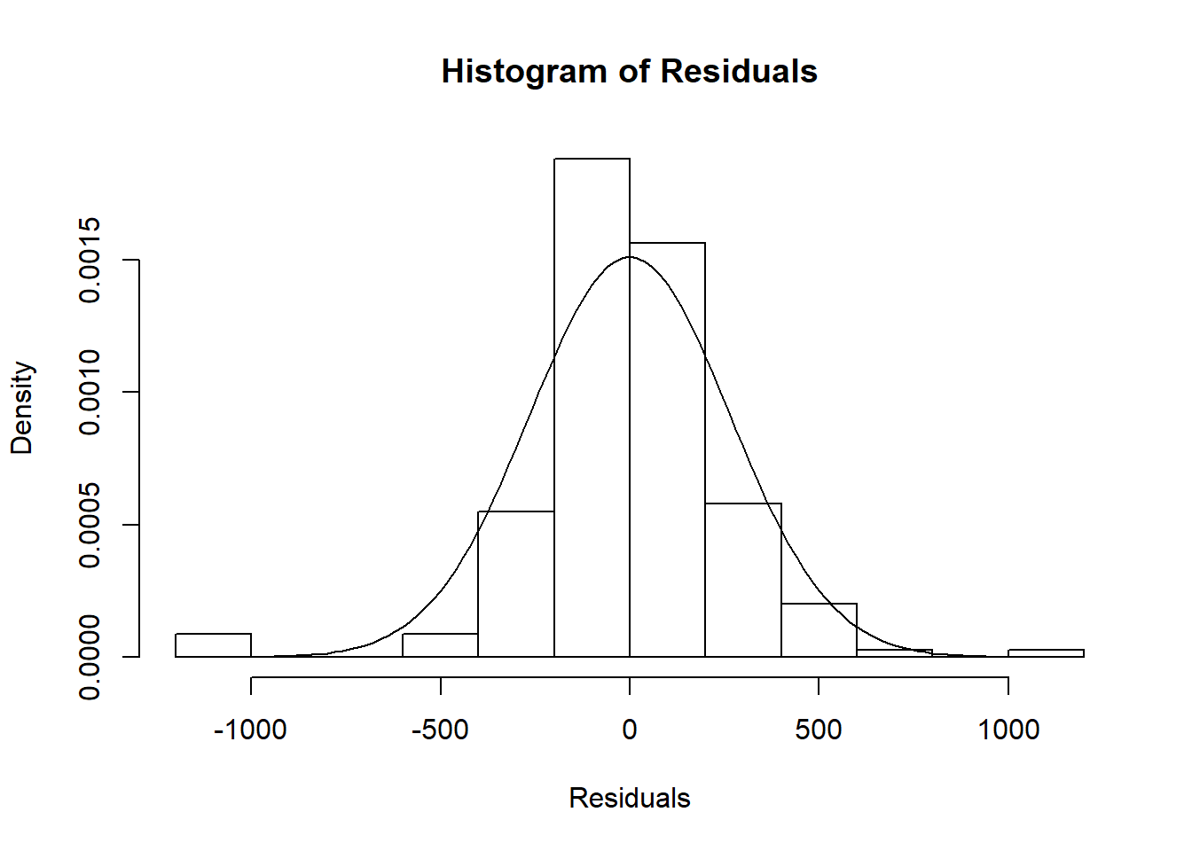

In the video I also mention the results of a Kolmogorov-Smirnov test of the residuals vs. a normal distribution.

ks.test(residuals(hsc1), "pnorm", 0, 264.1)

## Warning in ks.test(residuals(hsc1), "pnorm", 0, 264.1): ties should not be
## present for the Kolmogorov-Smirnov test

## 
##  One-sample Kolmogorov-Smirnov test
## 
## data:  residuals(hsc1)
## D = 0.089237, p-value = 0.1271
## alternative hypothesis: two-sided

Then there’s a quantile-quantile plot.

qqnorm(residuals(hsc1))
qqline(residuals(hsc1))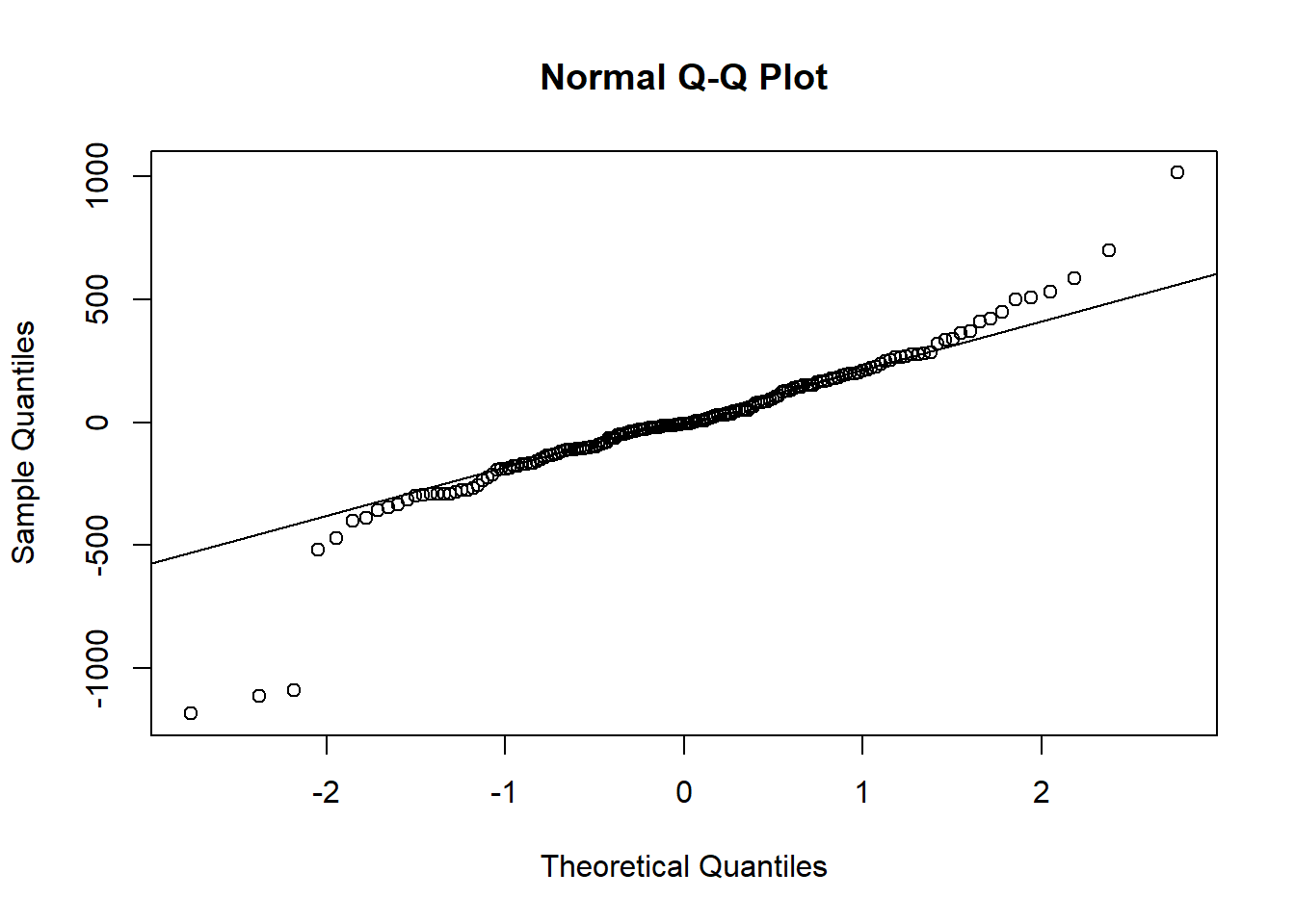

Next is the output of the plot() on a linear model object.

old.par <- par(mfrow = c(2,2))
plot(hsc1)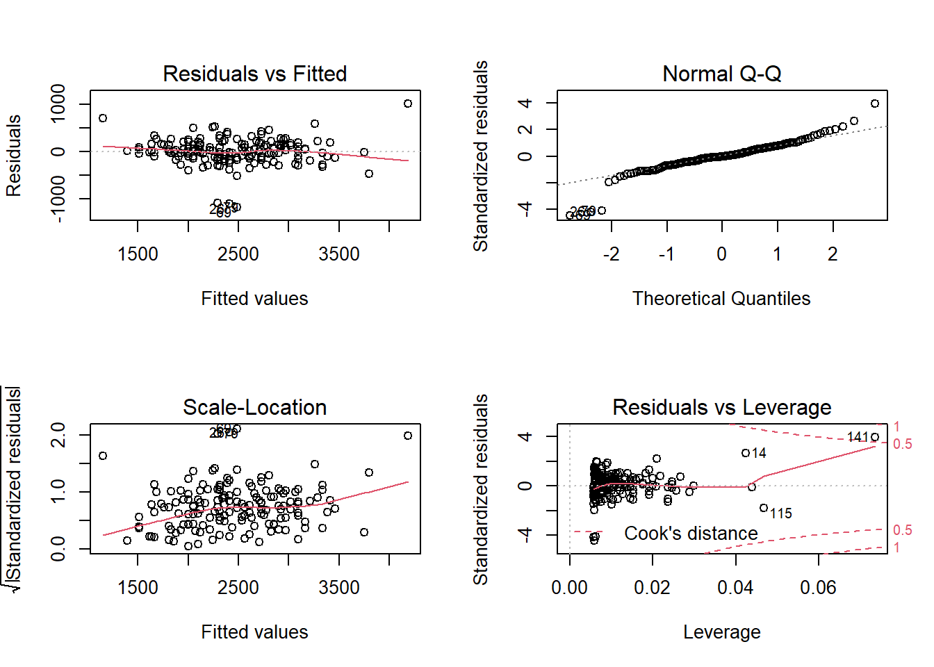

par(old.par)

My students and I put together a function that uses ggplot2 to make something similar. I like it because it includes confidence regions, which makes it easier to judge if the smooth spline is “flat”.

check_assumptions(hsc1)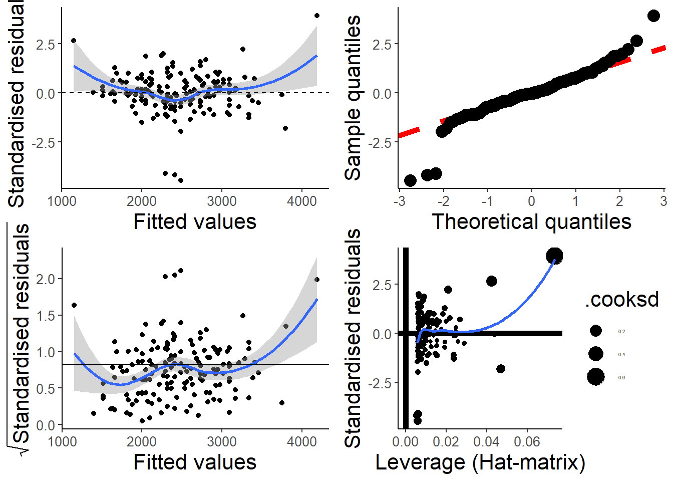

One thing that plot makes clear is the presence of several outliers. In The Ecological Detective, Ray Hilborn and Marc Mangel have an entire section entitled “Don’t let outliers ruin your life”. In that spirit, the next few plots identify and eliminate the outliers, and then refit the model. I’m going to switch over to using broom functions here, because too easy. I think in the video I remove the points with the largest absolute values of the residuals, which isn’t necessarily a good definition of an outlier.

crabs <- augment(hsc1) # add model diagnostics 
#which points have biggest residuals
crabs |>   ## native pipe!!
  rownames_to_column()|>
  arrange(desc(abs(.resid))) |>
  head()

## # A tibble: 6 x 9
##   rowname weight width .fitted .resid    .hat .sigma .cooksd .std.resid
##   <chr>    <int> <dbl>   <dbl>  <dbl>   <dbl>  <dbl>   <dbl>      <dbl>
## 1 69        1300  26.5   2486. -1186. 0.00583   252.  0.0581      -4.45
## 2 26        1300  26.2   2413. -1113. 0.00579   254.  0.0508      -4.18
## 3 79        1200  25.7   2292. -1092. 0.00625   255.  0.0528      -4.10
## 4 141       5200  33.5   4184.  1016. 0.0736    256.  0.618        3.95
## 5 14        1850  21     1151.   699. 0.0425    263.  0.158        2.67
## 6 91        3850  29.7   3262.   588. 0.0209    264.  0.0526       2.22

So rows 69, 26, 79, and 141 have large residuals, more than 50% larger than the remainder.

outliers <- c(26, 69, 79, 141)
hsc2 <- lm(weight~width, data = crabs[-outliers,])
plot(weight~width, data = crabs)
points(crabs[outliers,2, drop = TRUE], crabs[outliers,1, drop = TRUE], pch = "x", col = "red")
abline(hsc2, lwd = 2)
abline(hsc1, lty = 2)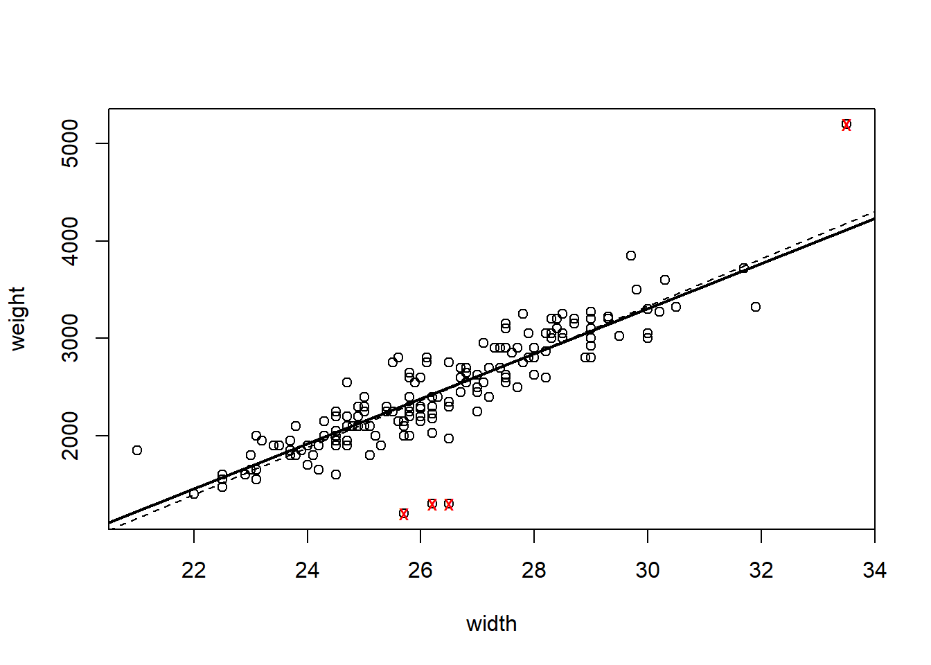

The “outliers” are identified with the red ’x’s. The original fit is given with a dashed line. How do the residual plots look with the outliers removed?

qqnorm(residuals(hsc2))
qqline(residuals(hsc2))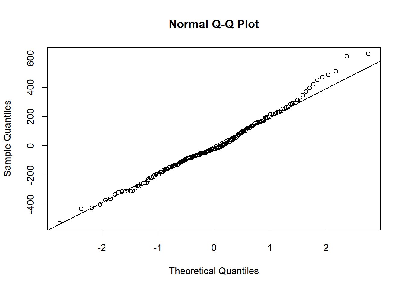

and checking for non-linearity by plotting residuals against the independent variable width.

plot(crabs[-outliers, "width", drop = TRUE], residuals(hsc2), 
     xlab = "width [cm]", ylab = "Residuals",
     main = "Residuals vs. Independent")
abline(h = 0, lwd = 2, lty = 2)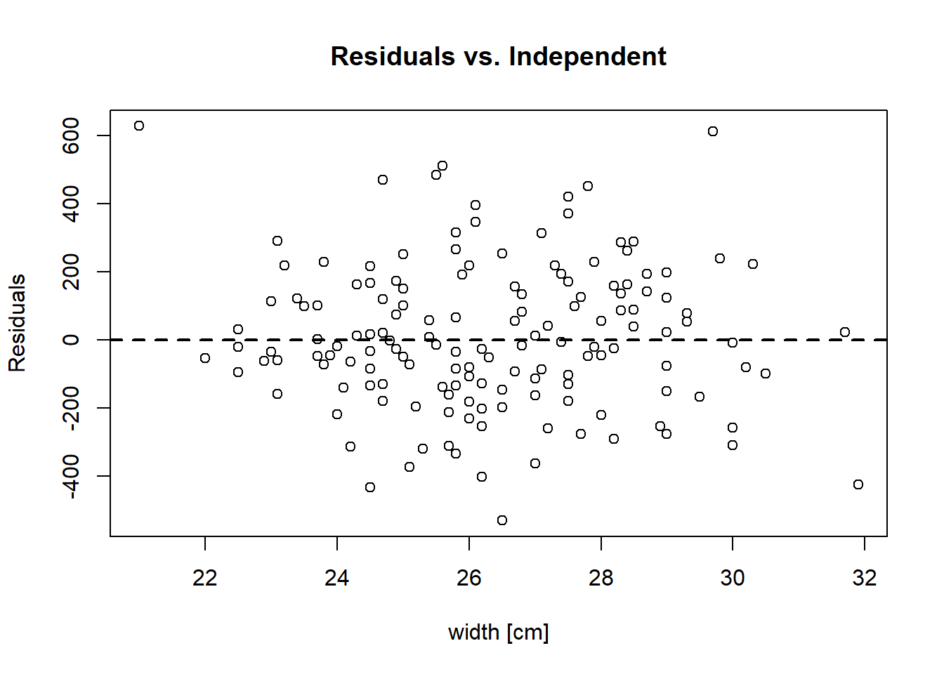

and finally with the function from my package.

check_assumptions(hsc2)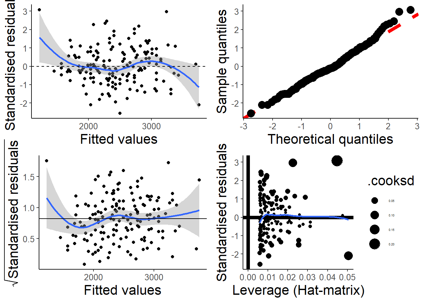

The scale-location plot in the bottom left also has a “guide” line at ~0.82, which turns out to be the expected value of the square root of the absolute value of the standardized residuals.

My students and I also developed a function that automatically plots the residuals against all the independent variables to check for possible non-linearities.

check_nonlinear(hsc2)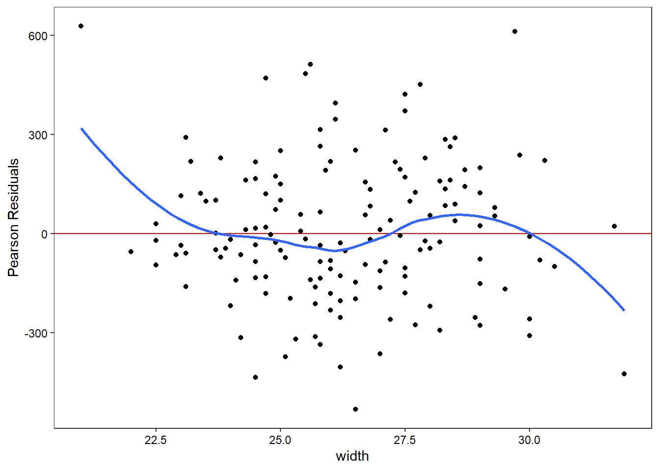

Hm. Clearly need to update that into ggplot for nice confidence regions!