Rethinking the logistic model

A few weeks ago I rambled on about carrying capacity as a concept. The day after I posted that, I stumbled across a paper by James Mallet in 2012 on why the r-K parameterization of the logistic model is all wrong. Mind Blown.

The essential point of the paper is that our typical form of logistic growth

\[ \frac{1}{N}\frac{dN}{dt} = r_{max}\left(1-\frac{N}{K}\right) \]

is a historical accident. Verhulst’s original form was

\[ \frac{1}{N}\frac{dN}{dt} = r_{max} - \alpha N \]

with an equilibrium population size given by \(N^* = r_{max} / \alpha\). This is brilliant, because now \(r_{max}\) represents growth in the absence of intraspecific competition, while \(\alpha\) is how much growth is reduced by intraspecific competition. Most importantly, these two parameters can vary independently. In contrast, \(r_{max}\) and \(K\) are linked at the hip.

To see this, consider the following diagram of per-capita birth and death rates changing with population size¹.

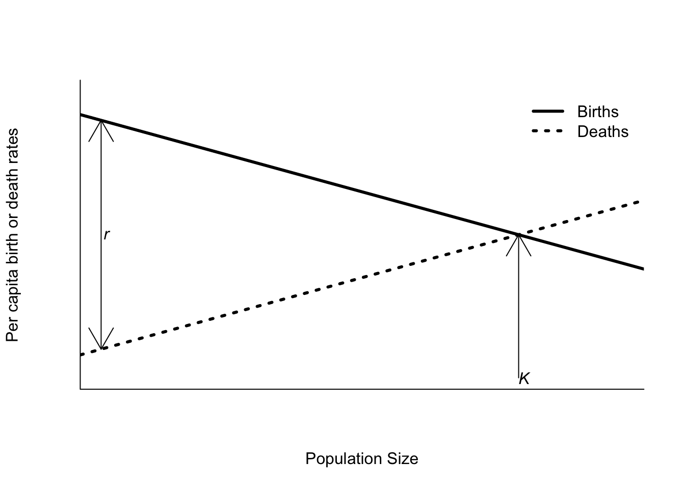
A change in per capita death rates, say by increasing trapping by humans that is density independent, shifts the death rate curve upwards, parallel to the current line. This reduces \(r_{max}\), because the y-intercepts get closer, and reduces \(K\), because now the two curves cross closer to the origin. However, \(\alpha\), the sum of the slopes of the lines does not change.

This isn’t a trivial side bar. Trevor Hefley’s work on detecting transcritical bifurcations in real populations ran into issues because of this non-independence. Trevor fit an r-K model to population data on Bobwhite. He allowed both \(r_{max}\) and \(K\) to change over time. If \(r_{max}\) dips below 0 while \(K > 0\), then the population goes through a “transcritical bifurcation” – the equilibrium population size ceases to exist, and the population decays exponentially towards 0. However, if \(N>K\) when the bifurcation occurs, the r-K model predicts an increase towards \(\infty\).

library("tidyverse")
library("tidypop") # note: code below using the dev branch of this package use
# devtools::install_github("atyre2/tidypop@dev") 

rKmod <- function(N0, r, K){
  N1 <- N0 + N0*r*(1-N0/K)
  return(N1)
}
inputs <- tibble(t = 1:20,
                 r = c(rep(0.5,10), rep(-0.1,10)),
                 K = c(rep(100,10), rep(90,10)))
outputs <- iterate(inputs, N0 = 20, rKmod)
ggplot(data = outputs,
       mapping = aes(x = t, y = N)) + 
  geom_line() + 
  geom_step(data = inputs,
            mapping = aes(y = K), linetype = 2)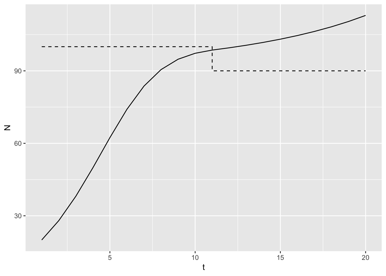

Needless to say that isn’t the expected behavior for \(r_{max} < 0\)! If I switch to the \(r-\alpha\) form, I need to work out what \(\alpha\) should be to have \(N^* = 100\). I think it is \(r/N^* = 0.005\) in this case so

ramod <- function(N0, r, alpha){
  N1 <- N0 + N0*r - alpha*N0^2
  return(N1)
}
inputs <- tibble(t = 1:20,
                 r = c(rep(0.5,10), rep(-0.1,10)),
                 alpha = 0.005,
                 K = r / alpha)
outputs <- iterate(inputs, N0 = 20, rKmod)
ggplot(data = outputs,
       mapping = aes(x = t, y = N)) + 
  geom_line() + 
  geom_step(data = inputs,
            mapping = aes(y = K), linetype = 2) + 
  ylim(c(0,100))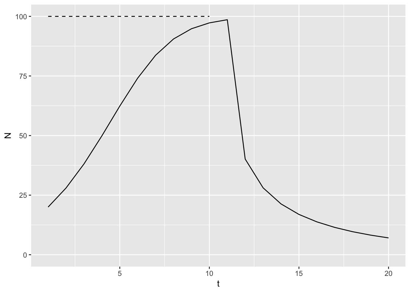

That’s more like it! The per capita effect of intra-specific competition didn’t change – the perturbation just affected the population in a density independent way.

What is \(\alpha\)? I’ll start with discrete time exponential growth, and substitute straight line functions for the per capita birth and death rates.

\[ \begin{align} N_{t+1} & =N_t\left(1 + b - d\right) \\ & =N_t + N_tb - N_td \\ & =N_t + N_t(b_0 + b_1N_t) - N_t(d_0 + d_1N_t) \\ & =N_t + N_t(b_0 - d_0) + N_t^2(b_1 - d_1) \\ & =N_t + r_{max}N_t -\alpha N_t^2 \end{align} \]

So \(b_0-d_0\) is usually rewritten as \(r_{max}\). But also, \(-\alpha = b_1 - d_1\), which is … just beautiful. To write that equation with \(K\) requires so much more algebra.

It also expands easily to competition. \[ \begin{align} N_{1,t+1} & =N_{1,t} + r_{max}N_{1,t} -\alpha_{11} N_{1,t}^2 - \alpha_{21}N_{1,t}N_{2,t} \\ N_{2,t+1} & =N_{2,t} + r_{max}N_{2,t} -\alpha_{22} N_{2,t}^2 - \alpha_{12}N_{2,t}N_{1,t} \end{align} \]

and so on! Wow.

Now I’ve even more reason to rewrite my lecture notes and redo all the videos. How do I check to see if this change improves student learning?