How big is too big: variance inflation factors

In a comment Jacob E. asked “Also, you mention using VIF for testing multi-collinearity. Is there a cutoff score you recommend for AIC?” I gave a snarky answer because I didn’t have a good answer. What would a good answer look like?

One way to proceed is to simulate data from the situation where the assumption is not violated, and look at the distribution of VIF scores.

library("tidyverse")

## -- Attaching packages --------------------------------------- tidyverse 1.3.1 --

## v ggplot2 3.3.3     v purrr   0.3.4
## v tibble  3.1.2     v dplyr   1.0.6
## v tidyr   1.1.3     v stringr 1.4.0
## v readr   1.4.0     v forcats 0.5.1

## -- Conflicts ------------------------------------------ tidyverse_conflicts() --
## x dplyr::filter() masks stats::filter()
## x dplyr::lag()    masks stats::lag()

n <- 100
N <- 1000
make_data <- function(beta = c(0, 0.1, 1, 10), sigma = 1, residual_error = 1, n = 1){
  if (is.null(dim(sigma))){
    tmp <- sigma
    sigma <- matrix(0, nrow = length(beta), ncol = length(beta))
    diag(sigma) <- tmp
  } 
  X <- MASS:::mvrnorm(n, mu = rep(0, length(beta)), Sigma = sigma)
  Y <- X %*% beta + rnorm(n, mean = 0, sd = residual_error)
  return(data.frame(Y, X))
}
#Test it out
test_df <- make_data(n = n)
ggplot(data = test_df,
       mapping = aes(x = X4, y = Y, color = X3)) + 
  geom_point()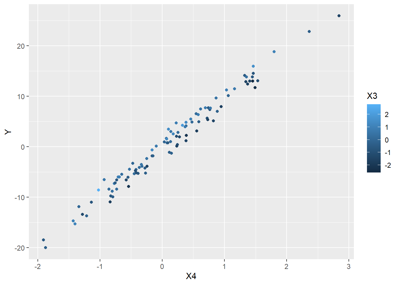

OK, now generate a bunch of data sets, fit linear models to them, and get the VIF scores.

vif_null <- map(1:N, ~make_data(n = n)) %>% 
  map(~lm(Y~X1+X2+X3+X4, data = .)) %>% 
  map_dfr(car::vif) %>% 
  mutate(rep = 1:N) %>% 
  pivot_longer(cols = -rep, names_to = "variable",values_to = "vif")
ggplot(data = vif_null,
       mapping = aes(x = vif)) + 
  geom_histogram() + 
  facet_wrap(~variable)

## `stat_bin()` using `bins = 30`. Pick better value with `binwidth`.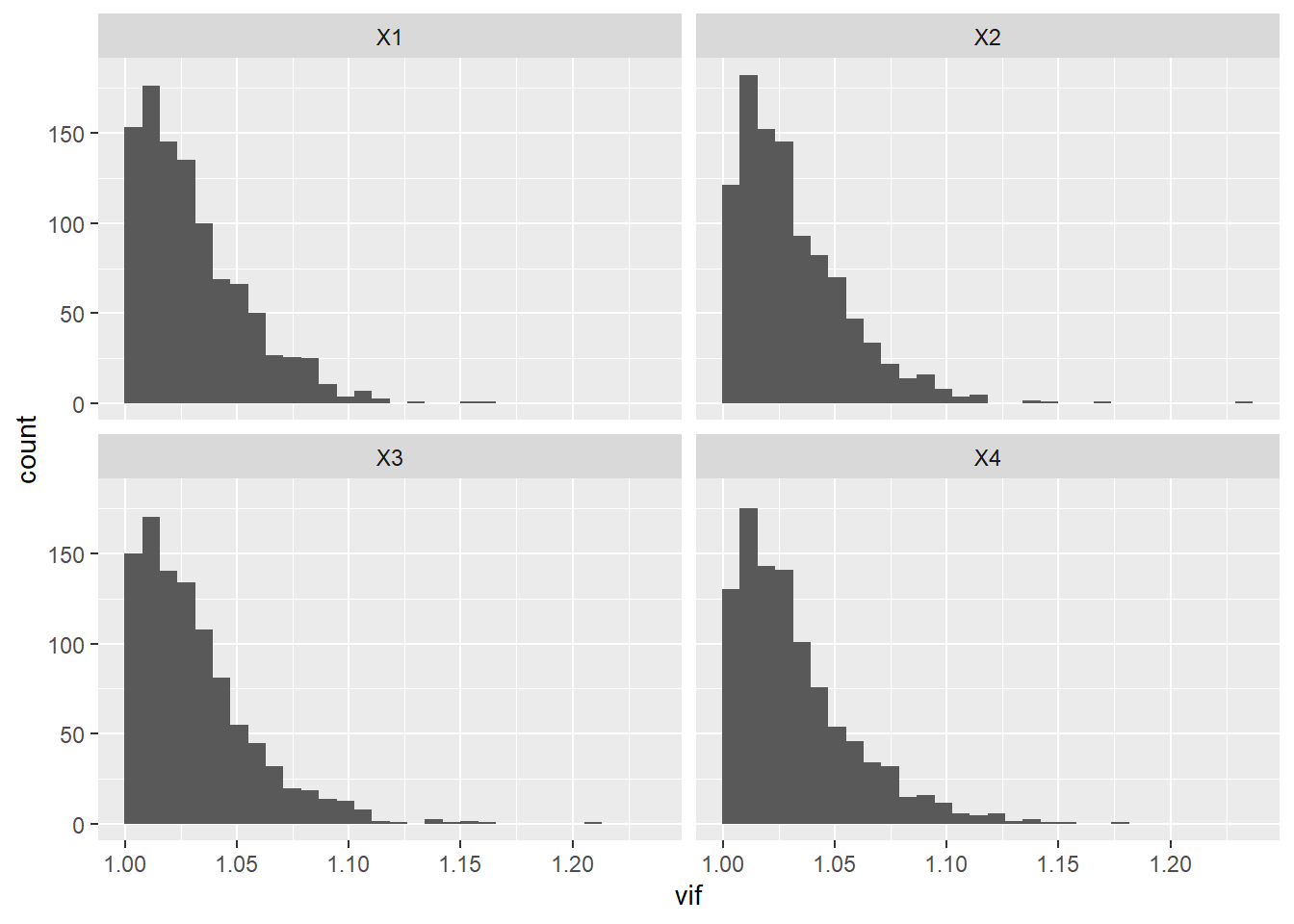

OK, wow! Didn’t expect that – if there is NO correlation between the predictor variables then VIF rarely exceeds 1.2. Lets do an example where a couple of the variables are highly correlated.

sigma <- matrix(c(1, 0, 0, 0,
                  0, 1, -0.9, 0,
                  0, -0.9, 1, 0,
                  0, 0, 0, 1), nrow = 4, ncol = 4)
vif_bad <- map(1:N, ~make_data(n = n, sigma = sigma)) %>% 
  map(~lm(Y~X1+X2+X3+X4, data = .)) %>% 
  map_dfr(car::vif) %>% 
  mutate(rep = 1:N) %>% 
  pivot_longer(cols = -rep, names_to = "variable",values_to = "vif")
ggplot(data = vif_bad,
       mapping = aes(x = vif)) + 
  geom_histogram() + 
  facet_wrap(~variable)

## `stat_bin()` using `bins = 30`. Pick better value with `binwidth`.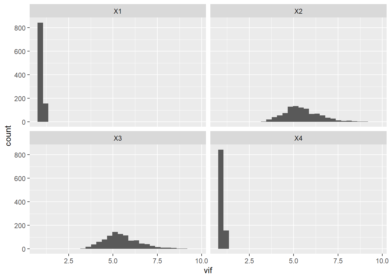

So a correlation of ~ -0.9 between two of the variables gives VIF scores bigger than 2, about 5 on average. So choosing a cutoff of 2 is going to exclude the worst offenders.