Today’s post represents a complete reset, because the data structures at the JHU repository changed Monday and haven’t fully settled down yet. Country level data are good; they haven’t got state level data for the USA anymore. Germany seems to be #flatteningthecurve. USA, Australia, and Canada are still on exponential growth curves.
The first post in this series was a week and a half ago, in case you’re just joining and want to see the progression.
EDIT 2020-10-14: Prof. Niko Speybroeck pointed out I’d made an error in the derivative (left out a minus sign) and copy/pasted the wrong df for the confidence limits in the first plot. No changes to the conclusions though. All fixed now! Thanks!
The bottom line
DISCLAIMER: These unofficial results are not peer reviewed, and should not be treated as such. My goal is to learn about forecasting in real time, how simple models compare with more complex models, and even how to compare different models.1
The figure below is complex, so I’ll highlight some features first. The y axis is now Active and Recovered cases / 100,000 population to make it easier to compare locales. The SOLID LINES are exponential growth models that assume the rate of increase is constant. The dashed lines are predictions from that model. The red rectangle shows the range of ICU bed capacity per 100,000 population in each country. The lower limit assumes all reported cases need ICU care (unlikely, but worst case). The top of the rectangle assumes only 5% of cases need ICU support. That best case assumes that the confirmed cases are a good representation of the size of the outbreak (also unlikely, unfortunately). Note that the y axis is logarithmic. The x axis is now days since the 100th case in each country.
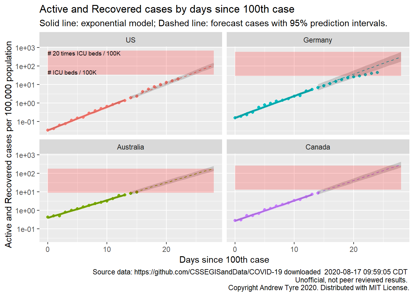
The most obvious feature on this plot is how the growth in cases is slowing in Germany. They are pulling this off with a massive testing effort that started early, in addition to getting people to move less. They are also reporting a very low death rate. Day 0 on this plot is the start of March for USA and Germany, and about March 10 for Canada and Australia.
If you’ve been following my earlier posts on the topic, you might notice that the prediction intervals on this figure are much, much narrower than previous plots. I’ve switched to plotting the cumulative “Active and Recovered” cases from the number of new cases per day. The variation (scatter around the line) is much smaller for the cumulative cases than new cases per day. That has two effects. First, the estimates of the growth rate become much more precise. Second, the smaller variability around the line directly reduces the variance of each future observation. These intervals are ignoring the correlation between one day and the next, so they are too narrow, but given that I am looking for the points to fall outside the intervals this is a conservative choice.
The other thing to remember is country level totals are obscuring significant variation, especially in the USA. Some states are already deep in the red zone (Louisiana, New York), while others like Nebraska have yet to show exponential growth. I don’t have up to date state level data to show this here, but hope to fix that soon.
The “recovered” data from JHU are full of missing values and other issues, because those numbers are not being reported consistently. I’ve calculated “Active and recovered” by subtracting deaths from confirmed cases. This is an overestimate of the load on the health care system, because people that recover are no longer a burden. Right now the number of recovered cases is low relative to new cases, but as the epidemic develops “Active and Recovered” will be worse as a estimate of health care burden.
Full Data Nerd
Jessica Burnett asked for regression statistics to be on each panel. That might be TMI for most people, but I could calculate the doubling time and add that to the plot.
\[ \begin{align} y_{t} = & y_{0}10^{bt} \\ 2y_{0} = & y_{t}10^{bt} \\ 2 = & 10^{bt} \\ t = & log_{10}(2)/b \end{align} \]
So I need to extract the slope estimate \(b\) from each regression. First fit all those models. This is the same code used for the figure above2.
library("tidyverse")
library("lubridate")
library("broom")
savefilename <- "data/jhu_wide_2020-03-26.Rda"

# The following code is commented out and left in place. This isn't particularly good coding
# practice, but I don't want to have to rewrite it every day when I get the updated data.
# I archive the data rather than pull fresh because this data source is very volatile, and
# data that worked with this code yesterday might break today.
# jhu_url <- paste("https://raw.githubusercontent.com/CSSEGISandData/",
#                  "COVID-19/master/csse_covid_19_data/",
#                  "csse_covid_19_time_series/time_series_covid19_",sep = "")
#
# jhu_confirmed_global <- read_csv(paste0(jhu_url,"confirmed_global.csv")) # just grab it once from github
# jhu_deaths_global <- read_csv(paste0(jhu_url,"deaths_global.csv")) # just grab it once from github
# jhu_recovered_global <- read_csv(paste0(jhu_url,"recovered_global.csv")) # just grab it once from github
# # archive it!
# save(jhu_confirmed_global, jhu_deaths_global, jhu_recovered_global, file = savefilename)
load(savefilename)

country_data <- read_csv("data/countries_covid-19_old.csv") %>%
  mutate(start_date = mdy(start_date))

only_country_data <- filter(country_data, is.na(province))
source("R/jhu_helpers.R")

# different data sources use different abbreviations for USA, and it is making me crazy.
countries <- c("US", "Australia", "Germany", "Canada")
countries2 <- c("United States", "Australia", "Germany", "Canada")
# Take the wide format data and make it long
all_country <- list(
  confirmed = other_wide2long_old(jhu_confirmed_global, countries = countries),
  deaths = other_wide2long_old(jhu_deaths_global, countries = countries)
  # recovered data is a mess lots of missing values
#  recovered = other_wide2long(jhu_recovered_global, countries = countries)
  ) %>%
  bind_rows(.id = "variable") %>%
  pivot_wider(names_from = variable, values_from = cumulative_cases) %>%
  # roll up to country level
  group_by(country_region, Date) %>%
  summarize(cumulative_confirmed = sum(confirmed),
            cumulative_deaths = sum(deaths)) %>%
  group_by(country_region) %>%
  mutate(incident_cases = c(0, diff(cumulative_confirmed)),
         incident_deaths = c(0, diff(cumulative_deaths)),
         active_recovered = cumulative_confirmed - cumulative_deaths) %>%
  left_join(only_country_data, by = "country_region") %>%
  mutate(icpc = incident_cases / popn / 10,
         arpc = active_recovered / popn / 10,
         group = country_region,
         date_100 = Date[min(which(cumulative_confirmed >= 100))],
         day100 = as.numeric(Date - date_100)) %>%
  ungroup() %>%
  mutate(country_region = factor(country_region, levels = countries))

# recreate this adding date_100
only_country_data <- all_country %>%
  group_by(country_region) %>%
  summarize(date_100 = first(date_100),
            popn = first(popn),
            icu_beds = first(icu_beds)) %>%
  mutate(max_icu_beds = icu_beds * 20,
         start_day = 0,
         end_day = 28)

all_models <- all_country %>%
  mutate(log10_ar = log10(active_recovered)) %>%
  filter(day100 <= 13, day100 >= 0) %>%  # model using first 2 weeks of data
  group_by(country_region) %>%
  nest() %>%
    mutate(model = map(data, ~lm(log10_ar~day100, data = .)))

all_fit <- all_models %>%
  mutate(fit = map(model, augment, se_fit = TRUE),
         fit = map(fit, select, -c("log10_ar","day100"))) %>%
  select(-model) %>%
  unnest(cols = c("data","fit")) %>%
  mutate(fit = 10^.fitted,
         lcl = 10^(.fitted - .se.fit * qt(0.975, df = 12)),
         ucl = 10^(.fitted + .se.fit * qt(0.975, df = 12)),
    fitpc = fit / popn / 10,
         lclpc = lcl / popn / 10,
         uclpc = ucl / popn / 10)

#all_predicted <- all_by_province %>%
all_predicted <- cross_df(list(country_region = factor(countries, levels = countries),
                               day100 = 14:28)) %>%
  #   mutate(day = as.numeric(Date - start_date)) %>%
  # filter(day > 12) %>% #these are the rows we want to predict with
  group_by(country_region) %>%
  nest() %>%
  left_join(select(all_models, country_region, model), by="country_region") %>%
  mutate(predicted = map2(model, data, ~augment(.x, newdata = .y, se_fit = TRUE)),
         sigma = map_dbl(model, ~summary(.x)$sigma)) %>%
  select(-c(model,data)) %>%
  unnest(cols = predicted) %>%
  ungroup() %>%
  left_join(only_country_data, by = "country_region") %>%
  mutate(
    Date = date_100 + day100,
    country_region = factor(country_region, levels = countries), # use factor to modify plot order
    fit = 10^.fitted,
All the model objects are in a “list column” called model. So now map() with broom::tidy() should
give us what we want.
all_models %>%
  mutate(estimates = map(model, tidy)) %>%
  unnest(cols = estimates) %>%  # produces 2 rows per country, (intercept) and day100
  filter(term == "day100") %>%
  select(country_region, estimate, std.error) %>%
knitr::kable(digits = 3)| country_region | estimate | std.error |
|---|---|---|
| Australia | 0.095 | 0.002 |
| Canada | 0.109 | 0.003 |
| Germany | 0.118 | 0.004 |
| US | 0.126 | 0.002 |
OK, so that’s what we want. However, one of my pet peeves is estimates/predictions without uncertainty
attached. So I also want to put confidence limits around the doubling time, and to do that I need
the variance of the doubling time. I have the variance (std.error^2) of the rate of growth.
I can use the Delta method to approximate the variance of doubling time. Everything I know about
the Delta method I learned from Larkin Powell.
He wrote an awesome how-to for the Delta method.
\[ var(\hat t) = var(\hat b)\left[\frac{\partial\hat t }{\partial \hat b}\right]^2 \\ \frac{\partial\hat t }{\partial \hat b} = -\frac{log_{10}2}{b^{2}} \\ var(\hat t) = var(\hat b)\frac{log_{10}2^2}{b^{4}} \]
doubling_times <- all_models %>%
  mutate(estimates = map(model, tidy)) %>%
  unnest(cols = estimates) %>%  # produces 2 rows per country, (intercept) and day100
  filter(term == "day100") %>%
  select(country_region, estimate, std.error) %>%
  mutate(var_b = std.error^2,
         t = log10(2) / estimate,
         var_t = var_b * log10(2)^2 / estimate^4,
         lcl_t = t - sqrt(var_t)*qt(0.975, 12),
         ucl_t = t + sqrt(var_t)*qt(0.975, 12),
         label = sprintf("%.2f (%.2f, %.2f)", t, lcl_t, ucl_t))

doubling_times %>%
  select(country_region, label) %>%
knitr::kable()| country_region | label |
|---|---|
| Australia | 3.16 (2.99, 3.33) |
| Canada | 2.77 (2.62, 2.91) |
| Germany | 2.56 (2.35, 2.76) |
| US | 2.38 (2.30, 2.47) |
Now make the plot, adding that in with a custom labelling function for the facets.
facet_labels <- doubling_times %>%
  mutate(label = paste0(country_region,", doubling time [days (95% CL)]: ", label)) %>%
  pull(label)
names(facet_labels) <- pull(doubling_times, country_region)
ggplot(data = filter(all_country, day100 >= 0),
                    mapping = aes(x = day100)) +
  geom_point(mapping = aes(y = arpc, color = country_region)) +
  facet_wrap(~country_region, dir="v", labeller = labeller(country_region = facet_labels)) +
  scale_y_log10() +
  theme(legend.position = "none",
        legend.title = element_blank()) +
  geom_line(data = all_fit,
            mapping = aes(y = fitpc, color = country_region),
            size = 1.25) +
  geom_ribbon(data = all_fit,
            mapping = aes(ymin = lclpc, ymax = uclpc),
            alpha = 0.2) +
  geom_line(data = all_predicted,
            mapping = aes(y = fitpc, color = country_region),
            linetype = 2) +
 geom_ribbon(data = all_predicted,
           mapping = aes(ymin = lplpc, ymax = uplpc),
           alpha = 0.2)  +
 geom_rect(data = only_country_data,
             mapping = aes(x = start_day, xmin = start_day, xmax = end_day, ymin = icu_beds, ymax = icu_beds * 20),
           fill = "red", alpha = 0.2) +
labs(y = "Active and Recovered cases per 100,000 population", title = "Active and Recovered cases by days since 100th case",
     x = "Days since 100th case",
       subtitle = "Solid line: exponential model; Dashed line: forecast cases with 95% prediction intervals.",
       caption = paste("Source data: https://github.com/CSSEGISandData/COVID-19 downloaded ",
                       format(file.mtime(savefilename), usetz = TRUE),
                       "\n Unofficial, not peer reviewed results.",
                       "\n Copyright Andrew Tyre 2020. Distributed with MIT License."))   +
  geom_text(data = slice(only_country_data, 1),
            mapping = aes(y = 1.4*icu_beds),
            x = 0, #ymd("2020-03-01"),
           label = "# ICU beds / 100K",
           size = 2.5, hjust = "left") +
    geom_text(data = slice(only_country_data, 1),
            mapping = aes(y = 20*icu_beds),
            x = 0, #ymd("2020-03-01"),
           label = "# 20 times ICU beds / 100K",
           size = 2.5, hjust = "left", vjust = "top")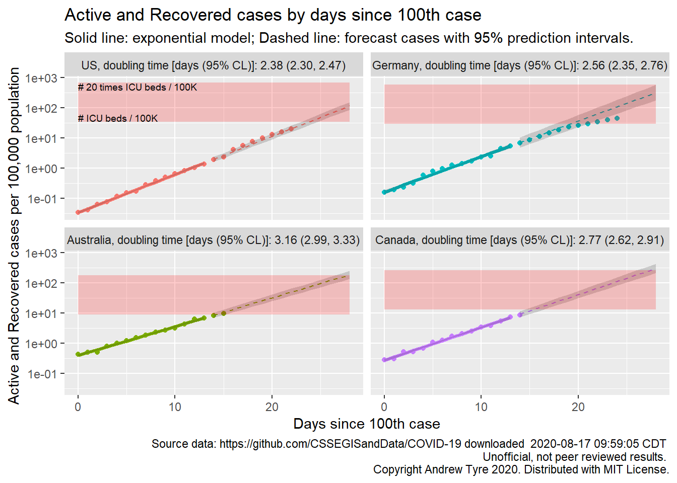
Woo! Keep in mind that’s based on the first two weeks after the 100th case, so in Germany the doubling time is currently increasing. Australian cases are growing the slowest, doubling about every 3 days. The initial growth rates in Germany and the USA might not be different (overlapping confidence limits).
What’s next?
So that’s enough for today. Hopefully this will quiet the peanut gallery (inside joke, sorry). Tomorrow I’ll try to find a dataset that includes states.
