I often hear the phrase, “This population is below \(K\) so …”. But what does the trajectory of such a population look like? I think it should be increasing. But apparently not everyone agrees. The usual context of this statement is interpreting what kind of birth and death rates to expect. If a population is “below \(K\)”, then birth rates should exceed death rates. If they are not, then something (disease, predation, hunting) is causing birth rates to fall or death rates to rise.
I’ve always thought of \(K\) as an abstract point, the position on the population size spectrum1 where birth and death rates are equal. In my thinking, if a disease arrives that reduces recruitment (e.g. by killing newborns), then \(K\) (and maybe \(r_{max}\)) is reduced because the birth rate curve shifts downwards. But apparently not everyone thinks of \(K\) in this arbitrary mathematical way.
I know there are many flavors of the term “carrying capacity”. For example, “social carrying capacity” as used by wildlife managers describes how many individuals of a species humans are prepared to accept.2 I think of my use of carrying capacity as “ecological carrying capacity”, the size of a population that growth tends towards in the absence of stochastic effects. But maybe this needs to be unpacked a bit more.
Thinking of \(K\) as a single thing creates a problem: my mathematical point does not stay constant. It bounces around in response to environmental stochasticity. In years with good rainfall \(K\) is higher for deer than in drought years. It trends over time in response to slow variables like landuse change. But the common usage suggests that \(K\) does not change. I think we need two concepts: \(K_t\) and \(K_{max}\).
\(K_t\) is the mathematical point I just described, and includes all the vagries of the environment, disease, predators etc. It is specific to a point in time and indeed, space. In contrast, \(K_{max}\) is constant, a feature of the species’ life history. In a given habitat3, at what population size do birth rates equal death rates equal given only intra-specific competition. In theory, one could work out \(K_{max}\) given knowledge of primary production, plant community composition, assimilation efficiencies, and assuming scramble competition. Here’s a graph to illustrate.
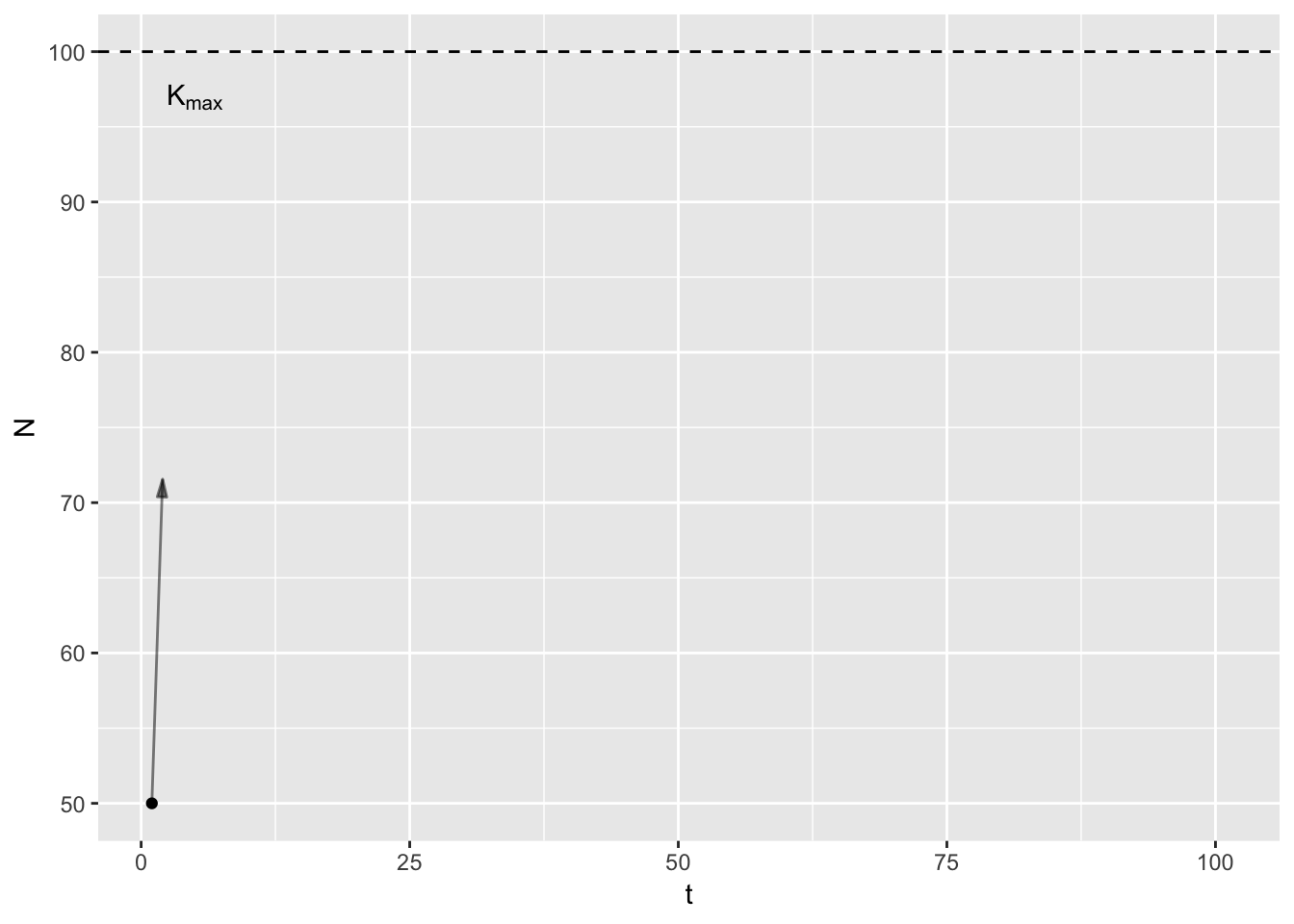
In the animation4, the arrows point from the current population size to \(K_t\), which varies randomly between years. Note that early on, the population increases even in bad years (years with low \(K_t\)), because the population is below \(K_t\).
I picked the \(K_{max}\) notation to correspond to \(r_{max}\), the intrinsic rate of growth, or the difference in birth and death rates when intra-specific competition is absent. This has a pleasing conceptual symmetry, but actually creates a problem. I use \(r_{max}\) in the sense of \(K_t\), that is, the maximum rate of growth including all the vagaries of the ecosystem. I use \(r_t\) as the observed per capita rate of growth at a particular point in time. So, if \(r_{max}\) is now the life history constant, \(r_t\) is the particular maximum growth rate at \(t\), then what is \(ln\left(\frac{N_{t+1}}{N_t}\right)\)?
My constants \(K_{max}\) and \(r_{max}\) have an interesting property. They are unobservable. Given two population estimates you can “observe” \(ln\left(\frac{N_{t+1}}{N_t}\right)\). By analogy with the distinction between population and sample statistics, I could use \(\rho_{max}\) for the life history constant, \(\rho_t\) for the value at a specific time, and then \(r_t = ln\left(\frac{N_{t+1}}{N_t}\right)\) just makes sense! Maybe. Conceptually \(r_t\) is not the same beast as \(\rho_t\) because the latter is independent of \(N_t\).
Getting this notation right is not a triviality. It affects how students learn. I’ve noticed many of my students struggle with this exact conceptual distinction between \(r_t\) and \(\rho_t\). One is an unobservable property of the system, and the other is an estimated quantity. Maybe I should put a hat on \(\hat{r}\). Another interesting connection: \(\hat{r}_t = f\left(\hat{N}_t | \rho_t, K_t\right)\).
Nothing to see here, really. I suspect the vague notation and terminology is so deeply engrained in generations of ecologists that clarifying it at this point is well nigh impossible. What do you think? Comments welcome below!
I just made this up. I love being an academic and getting to coin new jargon.↩
The concept is not without criticism - this is a fascinating read.↩
introducing another vague term here! Here, I think of habitat as a type of vegetation in a particular location, averaged at a resolution of at least the home range of the species in question. This works just fine for big horn sheep, but what about predators?↩
I assumed that \(K_t = K_{max} - gamma(10, 0.5)\) with shape and rate parameters for the gamma variate. You can see all the code if you’re keen.↩
