We’ll play with a few datasets from Mick Crawley’s “The R Book” 1 to see how to identify when a GAM can be useful, and when to stick with a GLM. The first dataset is of population sizes of Soay Sheep.
library(NRES803)
library(tidyverse)
library(mgcv)
library(broom)
library(GGally)
library(gridExtra)
# need this to make residual plots of gam models
bollocks.augment <- function(model) {
    r <- model.frame(model)
    r$.fitted <- fitted(model)
    r$.resid <- resid(model)
    r$.std.resid <- residuals(model, type = "scaled.pearson")
    r$.hat <- model$hat
    r$.cooksd <- cooks.distance(model)
    return(r)
}
data(sheep, package = "NRES803data")
ggplot(sheep, aes(x = Year, y = Population)) + geom_point()
The goal is to identify a function relating growth rate Delta to population size. The simplest population model has this as a linear function, but there’s no a priori reason to suppose that it should be linear.
sheep.lm <- lm(Delta ~ Population, data = sheep)
sheep.gam <- gam(Delta ~ s(Population), data = sheep)

# get residual df for both models
stuff_lm <- glance(sheep.lm)
stuff_gam <- glance(sheep.gam)

nd <- data.frame(Population = seq(600, 2000, 10))
pred_lm <- augment(sheep.lm, newdata = nd, se_fit = TRUE) %>%
    mutate(l95ci = .fitted - .se.fit * qt(0.975, stuff_lm$df.residual),
        u95ci = .fitted + .se.fit * qt(0.975, stuff_lm$df.residual)) %>%
    rename(Delta = .fitted)


pred.R <- predict(sheep.gam, newdata = nd, se.fit = TRUE)
pred.R <- as.data.frame(pred.R)
pred.R <- cbind(nd, pred.R)
names(pred.R)[names(pred.R) == "fit"] <- ".fitted"
names(pred.R)[names(pred.R) == "se.fit"] <- ".se.fit"
pred_gam <- pred.R %>%
    mutate(l95ci = .fitted - .se.fit * qt(0.975, stuff_gam$df.residual),
        u95ci = .fitted + .se.fit * qt(0.975, stuff_gam$df.residual)) %>%
    rename(Delta = .fitted)

# make a plot
ggplot(sheep, aes(x = Population, y = Delta)) + geom_point() +
    geom_line(data = pred_lm, color = "blue", size = 2) + geom_ribbon(aes(ymin = l95ci,
    ymax = u95ci), data = pred_lm, color = "grey", alpha = 0.33) +
    geom_line(data = pred_gam, color = "green", size = 2) + geom_ribbon(aes(ymin = l95ci,
    ymax = u95ci), data = pred_gam, color = "grey", alpha = 0.33)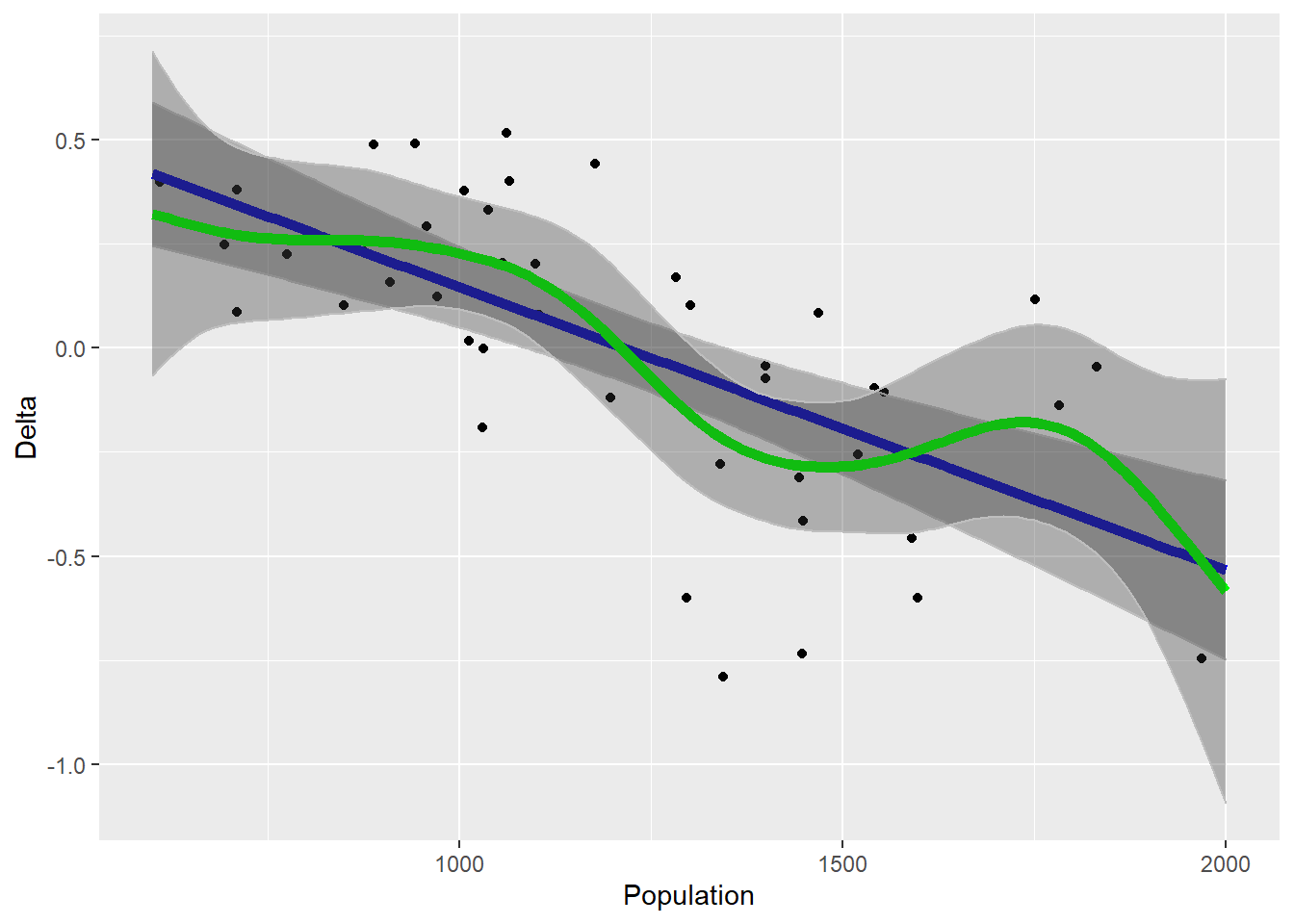
The gam fit is kind of interesting, looks like there are two broad regimes of population growth within which the growth rate is pretty constant with respect to population size. So which is the better model? This is actually quite important to get right, as the dynamics implied by the non-linear model will be much different. Recall that we can use gam() to fit the simpler model as well.
Check the assumptions graphically, and plot the residuals of both models against population size. Can you tell here which model is better? Would you use the linear or non-linear model, and why?
Fit the linear model using gam() and use anova() to compare the two models. Which one would you choose and why?
Ozone data
Next we’ll take a look at an air quality dataset. Not ecological, but a good test of your ability to see patterns in residuals.
The goal here is to predict ozone readings from solar radiation levels, temperature, and wind. You can see from the pairs plot that temperature in particular looks quite non-linear, as does radiation.
Set up a
gam()model with smooth terms for all three predictor variables. Evaluate this model graphically and interpret the results graphically (make a prediction plot) and in written form.log transform Ozone, and repeat the model with three smooth terms. Compare these two models graphically and numerically, choose which one is better, and explain why.
Based on your conclusions from the initial model, fit one or more new models with either fewer smooth terms (possibly linear), or additional interaction terms. Evaluate and interpret these models graphically and numerically.
